Pairwise Sequence Alignment: Revealing Genetic Differences and Similarities

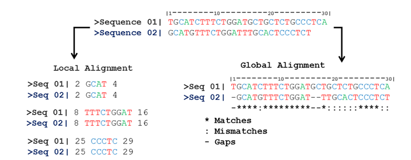
DNA and protein sequences undergo changes over time due to mutations. To investigate these evolutionary or environmental mutations or to identify biologically meaningful regions such as evolutionary relationships or functional similarities two or more biological sequences are compared. In these comparisons, individual bases or specific patterns are searched for. The process of arranging DNA or protein sequences one below the other and analyzing them to draw conclusions is called alignment (1). Alignment is classified into two types based on the number of sequences being compared: pairwise alignment and multiple sequence alignment. Pairwise alignment is used to determine the similarity between only two sequences. Additionally, alignment is further categorized as global or local, depending on its scope (2). In the following sections, we will explore what global and local alignment mean and in which contexts they are used. But first, let’s look at how alignment is performed and the criteria used to obtain meaningful results.

In alignment, scores are assigned based on the matching or mismatching of bases or amino acids starting from the ends of the two sequences. Gaps may be introduced to optimize the alignment. In a scoring system, matches are rewarded with positive scores, while mismatches and gaps are penalized. These scores are used to generate a numerical matrix that represents all possible alignments between the sequences. The highest scores in the matrix indicate the optimal alignments. One method for identifying these high-scoring alignments is dynamic programming, which efficiently finds the alignment with the highest score (3).

Figure 1. Alignment of Two Example Protein Sequences (3).

To perform more complex and biologically meaningful comparisons, substitution matrices are used. Two of the most commonly used examples are the PAM (Point Accepted Mutation) and BLOSUM (Blocks Substitution Matrix) matrices, which provide statistical data on how likely certain amino acid substitutions are from a biological perspective. These matrices allow for more accurate alignments by not only evaluating exact matches but also considering substitutions between evolutionarily similar amino acids (3).

Global alignment is a type of alignment in which the entire lengths of two biological sequences are compared from end to end. The goal of this algorithm is to find the best possible match throughout the entire length of the sequences. The Needleman-Wunsch algorithm, developed in 1970, was the first dynamic programming algorithm designed for this purpose. The algorithm constructs a scoring matrix and calculates the best score in each cell by considering possible scores from preceding cells. Scoring is based on matches, mismatches, and gap penalties (3). This method guarantees an optimal global alignment between sequences, but if the sequences contain many non-overlapping regions, it may not yield biologically meaningful results.

In contrast, local alignment focuses only on aligning the most similar region between two sequences. This type of alignment is particularly useful for identifying short conserved motifs or functional domains. The Smith-Waterman algorithm, developed in 1981, is the most widely used dynamic programming algorithm for local alignment. Like the Needleman-Wunsch algorithm, it also constructs a scoring matrix, but negative scores are replaced with zero, and only high-scoring regions are traced (3). As a result, the rest of the sequences are excluded from the alignment, and biologically meaningful local matches can be identified.

Figure 2. Global and Local Alignments of DNA Sequences (2).

Although dynamic programming methods offer high accuracy, they require increased computation time and memory for long sequences. Therefore, faster yet approximate methods like FASTA and BLAST have been developed. The working principle of FASTA is based on dividing the sequence into short fixed-length subsequences (k-tuples). These subsequences are matched with sequences in the target database, and then detailed alignment is performed. BLAST, on the other hand, breaks the query sequence into short words and searches the database for matches. Matching regions are extended, scores are calculated, and high-scoring alignments are identified.

Needleman-Wunsch Algorithm

One of the first and most important algorithms developed for aligning protein sequences was introduced by Needleman and Wunsch in 1970 (4). This algorithm is significant because it allows for the insertion of gaps in the alignment of protein or DNA sequences to provide the optimal alignment. While the result is optimal, it does not require evaluating all possible alignments—since performing an exhaustive pairwise comparison would be computationally expensive, demanding excessive time and processing power (5).

Global sequence alignment using the Needleman–Wunsch algorithm can be explained in three steps:

1. Matrix Initialization

2. Scoring the Matrix

3. Determining the Optimal Alignment

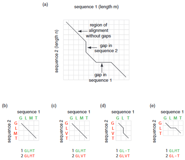
Step 1 – Matrix Initialization: First, the two sequences are compared within a two-dimensional matrix (Figure 3.). The first sequence, of length m, is placed horizontally along the x-axis, so that its amino acid residues correspond to the columns. The second sequence, of length n, is placed vertically along the y-axis, where its amino acid residues correspond to the rows.

Figure 3. Pairwise alignment of two amino acid sequences using the dynamic programming algorithm for global alignment developed by Needleman and Wunsch (1970). (a) The two sequences can be aligned along a diagonal path through the matrix, which may deviate horizontally or vertically when necessary; such deviations indicate the insertion of gaps into the alignment. (b) When the two sequences are completely identical, the alignment path follows a straight diagonal line across the matrix. (c) If there is a mismatch—or multiple mismatches—the path still generally follows a diagonal direction; however, a scoring system penalizes such mismatches (i.e., assigns lower scores). (d) If the alignment contains a gap in the first sequence, the path includes a vertical line. (e) If the alignment contains a gap in the second sequence, the path includes a horizontal line (5).

A perfect alignment between two identical sequences is represented by a straight diagonal line extending from the top-left to the bottom-right corner of the matrix (Figure 3a, b). Even if there are mismatched positions between the two sequences, the alignment still follows a diagonal path (Figure 3c). However, the score given for such matches can be adjusted based on a scoring system. For example, the mismatch between residues V and M in Figure 3c would receive a lower score compared to the perfect match between M and M in Figure 3b. If the alignment includes a gap, it is represented as a vertical line when the gap occurs in the first sequence (Figure 3d), or as a horizontal line when the gap is in the second sequence (Figure 3e). Any gap in the lower sequence is shown as a horizontal line (Figure 3e). These gaps can be of any length and may appear either internally or at the ends of the sequence (5).

Step 2 – Scoring the Matrix: The goal of this algorithm is to determine the optimal alignment. To do so, two matrices are created: an identity matrix and then a scoring matrix. The dimensions of the matrix are defined as (m + 1) × (n + 1), corresponding to the lengths of the first and second sequences along the x- and y-axes (Figure 4a). Gap penalties (in this case, –2 for each gap position) are assigned to the first row and column. This allows for the inclusion of terminal gaps of any desired length. Next, the identity positions are filled in (Figure 4a, grey-filled cells); this is referred to as the identity matrix. When two sequences are completely identical, a continuous diagonal line of grey-filled cells appears across the matrix. Then, a scoring system is defined (Figure 4b). The goal of finding the optimal alignment is to identify the path through the matrix that yields the highest possible score. This means finding a path that contains the maximum number of identity positions while introducing the minimum number of gaps (5).

Figure 4. The algorithm developed by Needleman and Wunsch (1970) can be used for the global alignment of two amino acid sequences. For this, a matrix of dimensions (m + 1) × (n + 1) is created based on the lengths of the two sequences, m and n. After constructing this matrix, the cells are filled using a specific scoring system. For example, +1 is assigned for matches, –2 for mismatches, and –2 for gap penalties. The score in each cell, F(i, j), is calculated from three possible options: the first is coming from the top-left diagonal cell (representing a match or mismatch), the second is coming from the cell to the left (with a gap penalty applied), and the third is coming from the cell above (again with a gap penalty).

At each position i, j (Figure 4b.), there are four possibilities:

1.The two residues may match exactly (i.e., be identical); in this case, +1 point is given for the match.

2.The residues may not match (be mismatched); in this case, –2 points are given.

3.A gap can be added to the first sequence; this results in –2 points.

4.A gap can be added to the second sequence; this also results in –2 points.

The Needleman-Wunsch algorithm assigns a score for each of these possible situations at each position in the aligned sequences. It also provides a set of rules defining how to move through the matrix. When considering the bottom-right cell in Figure 4c., there are several rules for deciding the optimal score:

1.First, both i and j should increase. Therefore, the scores from three positions (top, left, and top-left diagonal) are evaluated for a specific cell F(i, j). This is necessary to maintain the linear arrangement of amino acids (or nucleotides) in a sequence.

2.Gaps can be extended to the desired number of positions; the scoring system may include separate penalties for gap creation and gap extension.

3.The given score can come from a scoring matrix like BLOSUM62.

When beginning the alignment of the two sequences in the example, a score of +1 is assigned to a cell due to the alignment of the two F residues (Figure 4d.). Alternative options (such as adding a gap to either sequence) result in a lower score because they incur a gap penalty. The preferred (highest-scoring) path is shown with a red arrow throughout Figure 4. Next, the algorithm moves to the next cell on the right and selects a score of –1 (from the left cell: previous cell +1, gap penalty –2 → total of –1). This is better than the alternative scores of –4 and –6 (Figure 4e.). This process of analyzing the possible scores for each cell continues across each row (Figure 4f.), and eventually, the entire matrix is filled (Figure 4g.) (5).

Step 3 – Determining the Optimal Alignment: Once the matrix is filled, the alignment is determined using the trace-back method. This process starts from the bottom-right corner of the matrix (for proteins, the C-terminal or for nucleic acids, the 3' end). In this example, the score in this cell is –4, corresponding to the alignment of two glutamate residues. For this and all other cells, the best score can be traced back to one of the three neighboring cells. This process is summarized in Figure 5a.; the red arrows show the direction from which the highest score came. This defines a path that corresponds to the actual alignment (shown with orange-colored cells). In Figure 5b., arrows indicate the cells from which the best score came, providing an alternative way to define the optimal pairwise alignment (5).

Figure 5. The global pairwise alignment of two amino acid sequences is performed using the dynamic programming algorithm, with matrix scoring and the alignment obtained through the trace-back method. In the alignment shown in Figure 4g, the cells highlighted in pink represent the sources of the optimal scores. In an equivalent representation, arrows indicate the cell from which each cell's best score was derived. This trace-back process allows us to determine the optimal alignment's sequence. Vertical or horizontal arrows represent positions where gaps were added to the alignment, while diagonal lines represent exact matches or mismatches. The final score of –4 is the total score of matches, mismatches, and gaps. In this example, there are 6 matches (6 × +1 = +6), no mismatches, and 5 gaps, which contribute a total of –10 points (5 × –2 = –10). The sum of these values is –4, which is the total score of the alignment (5).

In this way, an alignment is created by progressing from the C-terminal to the N-terminal while including the gaps in both sequences. The final alignment obtained (Figure 5c) is absolutely optimal according to the scoring system used. Although it is rare, in some cases, multiple alignments may share the same optimal score, but this is quite uncommon when scoring matrices like BLOSUM62 are used (5).

Smith-Waterman Algoritması

The Smith-Waterman algorithm, developed by Smith and Waterman (1981) (6), is an important method for performing local alignment of two protein or DNA sequences. Local alignment is particularly useful in applications where only certain regions of proteins (not the entire sequences) are aligned, such as in database searches. The local sequence alignment algorithm works similarly to global alignment: two sequences (either protein or DNA) are placed into a matrix, and the optimal path is searched along the diagonal. However, in local alignment, the alignment can begin anywhere within the sequences, and it does not necessarily extend to the ends of the sequences—meaning the start and end points are free to vary. For the Smith-Waterman algorithm, an additional row is added at the top of the matrix, and an additional column is added on the left side to form the matrix. When the lengths of the sequences are m and n, the size of the matrix is (m + 1) × (n + 1). The rules for scoring each position in the matrix are slightly different from those used in the Needleman-Wunsch algorithm.

In this algorithm, the score for each cell is chosen from the highest value among the previous diagonal, left, or top cells after considering the possibility of adding a gap. However, an important rule in the Smith-Waterman algorithm is that the score can never be negative. If all possible values result in a negative score, the corresponding cell is assigned a score of zero (0). In other words, the S(i,j) score is defined as the highest value from the following four possibilities:

1.The score from the diagonal cell at position (i – 1, j – 1), with the score for the current position s[i, j] being a match or mismatch.

2.The score from the left cell S(i, j – 1), adjusted by subtracting a gap penalty.

3.The score from the top cell S(i – 1, j), also adjusted by subtracting a gap penalty.

4. Zero (0). (5).

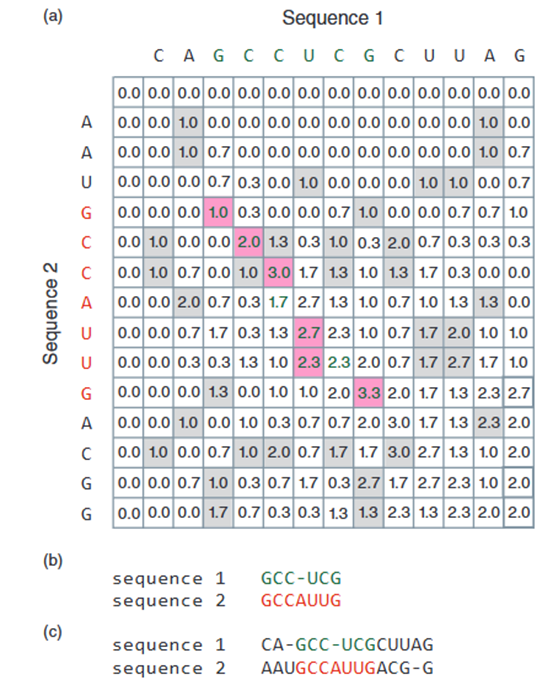
This condition ensures that negative values are never present in the matrix. In contrast, negative numbers are commonly found in global alignments due to gap and mismatch penalties. An example of aligning two nucleic acid sequences using the local alignment algorithm (adapted from Smith and Waterman, 1981) is shown in Figure 5. The top row and leftmost column of the matrix are filled with zeros. The maximum alignment can start and end anywhere within the matrix (5).

Figure 6. (a) In this example, the matrix is constructed from two RNA sequences (CAGCCUCGCUUAG and AAUGCCAUUGACGG). This is not an identity matrix, but positions where nucleotide matches occur are colored grey (or pink in the local alignment region). The scoring system used here is as follows: +1 for matches, –1/3 for mismatches, and the gap penalty is the difference between match and mismatch (a 1.3 gap penalty when the gap length is 1). The matrix is scored by selecting the largest of the four possible non-negative values. The highest value in the matrix (3.3) is the starting point of the optimal local alignment, and the aligned nucleotides (shown in green text) continue upwards and leftwards until they reach a value of zero. (b) The local alignment derived from this matrix is shown. This alignment contains matches, a mismatch, and a gap. (c) For comparison, the global alignment of the two sequences is also shown. This alignment covers the entire length of both sequences (6).

The path to follow is to identify the highest value in the matrix (in Figure 5a, this value is 3.3). This value represents the endpoint of the alignment (the 3' end for nucleic acids or the C-terminal for proteins). This position does not have to be in the bottom-right corner of the matrix, as it would be in global alignments. The trace-back process starts from this highest-value cell and moves diagonally upwards and to the left, continuing until it reaches a cell with a value of zero. This point defines the start of the alignment and does not have to be in the top-left corner of the matrix.

Pairwise sequence alignment is one of the fundamental tools in bioinformatics for determining similarities between biological sequences and translating these similarities into functional, structural, or evolutionary insights. The Needleman-Wunsch and Smith-Waterman algorithms, which are used for global and local alignment respectively, are considered reference methods due to their high accuracy. However, with the increasing volume of data, faster methods like dotplot, FASTA, and BLAST have become indispensable in practical applications. While all these methods address different needs in the interpretation of biological data, the choice of the correct alignment strategy should depend on the goals of the study, the type of data, and available resources.

References

1. Haubold, B., & Wiehe, T. (2006). Introduction to computational biology: An evolutionary approach. Birkhäuser Verlag.

2. Diniz, W. J. S., & Canduri, F. (2017). Bioinformatics: An overview and its applications. Genetics and Molecular Research, 16(1), gmr16019645. https://doi.org/10.4238/gmr16019645

3. Mount, D. W. (2004). Bioinformatics: Sequence and genome analysis (2nd ed.). Cold Spring Harbor Laboratory Press.

4. Needleman, S. B., & Wunsch, C. D. (1970). A general method applicable to the search for similarities in the amino acid sequence of two proteins. Journal of molecular biology, 48(3), 443–453. https://doi.org/10.1016/0022-2836(70)90057-4

5. Jonathan Pevsner. (2009). Bioinformatics and Functional Genomics. John Wiley & Sons, Inc. https://doi.org/10.1002/9780470451496

6. Smith, T. F., & Waterman, M. S. (1981). Identification of common molecular subsequences. Journal of molecular biology, 147(1), 195-197.