Molecular Mechanics’ Cornerstone: Force Fields – Part 1

Molecular modeling aims to simulate natural physical processes in a computer environment by numerically describing interactions between atoms. One of the fundamental building blocks of this process, force fields, are sets of mathematical functions and parametric constants that define how atoms interact with one another. Through force fields, molecular geometries can be optimized. In this optimization process, bonds are stretched, angles are bent, and the system’s energy is calculated. However, the accuracy of a force field is directly related to the quality of the parameters used. This is where the parameterization process comes into play. Using data obtained from experimental results or quantum chemical calculations, these parameters are adjusted to achieve consistency. In this article, we will explore in detail the basic principles of force fields and the parameters used within them.

Force Fields

Most classical force fields are based on five fundamental elements described through simple physical interpretations. These elements include potential energy terms associated with bond deformation and angle geometry (stretching and bending angles), as well as terms representing torsions around specific dihedral angles. In addition, there are free terms describing electrostatic interactions, dispersion interactions and repulsion when atoms come together (e.g., van der Waals forces). A force field consists of equations selected to model potential energy and the relevant parameters (1). The force field is the potential energy function used to describe the relationship between the structure (R) and the energy (U) of the system of interest. However, the potential energy function alone does not constitute a force field. A force field arises from the combination of the potential energy function with the parameters used in that function, as shown below (1).

Equation (1)

Equation (1) provides an example of what is called the total potential energy function. As can be seen, Equation (1) consists of a set of simple functions representing the minimal set of forces capable of describing molecular structures. Bonds, angles, and out-of-plane distortions (improper dihedral angles) are treated harmonically, while dihedral or torsional rotations are described using a sinusoidal term.

Interactions between atoms employ the 12–6 Lennard-Jones (LJ) term to describe atom–atom repulsion and dispersion interactions, combined with electrostatic interactions processed through the Coulombic term. In Equation (1), b is the bond length, Θ is the valence angle, χ is the dihedral angle, ϕ is the improper angle, and rij is the distance between atoms i and j. The parameters representing the actual force field terms include the bond force constant and equilibrium bond distance (K_b and b₀), the valence angle force constant and equilibrium angle (K and Θ), the dihedral force constant, multiplicity, and phase angle (Kχ, n, and δ), and the improper force constant and equilibrium improper angle (K and ϕ₀) (1).

Collectively, these represent the intramolecular parameters. The nonbonded parameters between atoms i and j include the partial atomic charges (qi) used for van der Waals (vdW) interactions, the LJ potential well depth, and the minimum interaction radius.

Intramolecular Parameters (Bonded Interactions)

Bond Length Potentials

Bond length potentials can be considered “strain” terms that model small-scale deviations around reference values. Reference values for different chemical bonds can be obtained from X-ray crystal structures or from quantum mechanical solutions of the equilibrium structures of small molecules (2).

1. Harmonic Term

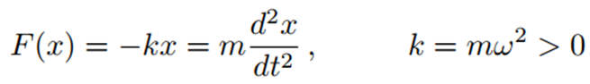
The harmonic potential, modeled using Hooke’s Law, is the simplest molecular mechanics approach used to describe bond deformations. According to Hooke’s Law, the force (F) is proportional to the displacement (x) and the acceleration (ẍ). This relationship can be expressed as:

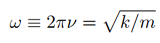
For this reason, the angular frequency ω (the number of radians per unit time) or equivalently, 2π times the circular frequency ν (where ν = c/λ, c is the speed of light, and λ is the wavelength) is related to the spring constant k as follows:

The corresponding potential energy (E) is given by:

More generally, this harmonic bond potential can be written as:

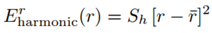
Here, r denotes the bond length, r̄ is the reference (equilibrium) bond length, and S_h​ represents a constant coefficient.

The harmonic potential is sufficient only for small deviations from the reference values. This usually applies to one vibrational level above the ground state or to length deformations of about 0.1 Å or less. It is not valid for larger deviations because, in that case, the atoms dissociate and no longer interact. Therefore, instead of increasing rapidly beyond the distance r̄, the energy levels off. However, at very short interaction distances, the deformation energy becomes extremely large (2).

2. Morse Term

To model bond deformations that go beyond very small oscillations around equilibrium states, the empirical bond potential developed by P.M. Morse (3) has proven to be quite successful in reproducing the vibrational levels of small molecules (4). The mathematical form of the Morse function is as follows:

The adjustable parameters S_m​ and D define the width and depth of the potential well, respectively. The Morse potential accurately reflects the rapid increase in energy when the bond length shortens (as r → 0, E(r) → ∞), but at large r values, the energy levels off and approaches the dissociation energy D (as r → ∞, E(r) → D).

Figure 1. Morse, harmonic, cubic, and two different quartic bond potentials for the HBr compound (2).

3. Cubic and Quartic Terms

To better reproduce Morse potentials beyond what can be achieved with the harmonic potential, cubic and quartic polynomials can be used (these are added terms to the second-degree potential). For example, the MM3 force field employs cubic and quartic bond potentials that work well for most molecules (5). The Merck force field, MMFF (6), uses a quartic bond function. The coefficients of the polynomial can be adjusted to better optimize the shape of the bond length potential function.

For large-molecule force fields, where computational time is critical, a special quartic potential has been proposed to avoid square root calculations (7); this measures the square of the squared bond length differences as follows:

Bond Angle Potentials

The bond angles around each atom in a molecule are determined by the hybridization of the orbitals around that atom (you can find more details about hybridization by clicking this link.). This rule serves as an initial estimate for bond angle geometries. However, small deviations often occur from these estimates, and sometimes larger deviations can arise. Even small differences of 1–2° between different bond angles in a molecule can have significant global effects on the molecular structure, such as in ribose (2).

1. Harmonic and Trigonometric Terms

Commonly used bond-angle potentials are harmonic functions involving the difference between angles and the cosine of angles. They can be defined by the following equations.

The advantage of the trigonometric potential is that it is bounded and can be easily applied and differentiated. This is because there is no need to compute inverse trigonometric functions, and it helps prevent singularity problems that may arise for linear bond angles.

Figure 2. Harmonic bond-angle potentials for an aromatic C–C–C bond angle (CA–CA–CA atom sequence in CHARMM) (2).

2. Cross Terms Between Bond Stretching and Angle Bending

Cross terms are frequently used in force fields designed for small molecular systems (e.g., MM3 and MM4). This is to more accurately model compensatory tendencies in bond lengths and bond angle values. These cross terms are considered correction terms to the bond length and bond angle potentials. For example, a stretch/bend term for the bonded atom sequence abc allows the a–b and b–c bond lengths to increase as the θ_abc angle decreases, or to decrease as the θ_abc angle increases. A bend/bend potential appropriately correlates the bending vibrations of two angles around the same atom. This separation of the relevant frequencies allows for better agreement with experimental vibrational spectra (5). These correlations can be modeled with stretch/stretch, bend/bend, and stretch/bend potentials for abc sequences. Here, r and r′ distances are associated with the ab and bc bonds, respectively, and θ represents the abc bond angle (2).

Torsional Potentials

1. Fourier Terms

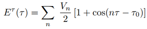
The general function used for each flexible torsion angle (τ) is of the following form, where n is an integer:

For each torsional sequence defined by the torsion angle τ, the integer n represents the periodicity of the rotational barrier, and Vₙ corresponds to the height of that barrier. The value of n used for each torsional degree of freedom depends on the atomic sequence and the force field parameterization. Typical values for n are 1, 2, and 3 (sometimes 4), while some force fields (such as CHARMM (8)) also use other values like n = 5 or 6. A reference torsion angle τ₀ can also be included in the formula.

Experimental data obtained from spectroscopic methods suitable for various spectral regions such as NMR, IR (Infrared Radiation), Raman, and microwave can be used to estimate barrier heights and periodicities in low molecular weight compounds. Since barriers to rotation around various single bonds in nucleic acids and proteins cannot be obtained experimentally, they should be estimated from similar chemical sequences in low molecular weight compounds (2).

In this article, we have examined in detail the internal structure of force fields, one of the fundamental building blocks of molecular modeling, focusing especially on intrinsic parameters such as bond lengths and angle bending. The accuracy and effectiveness of force fields are directly dependent on the quality of the parameterization used. Therefore, it is of great importance to carefully optimize the parameters by utilizing both theoretical and experimental data. In the next section of the article, we will focus on nonbonded forces between molecules (van der Waals interactions and electrostatic forces) and elaborate on the role of these interactions in molecular modeling.

References

1. Mackerell A. D., Jr (2004). Empirical force fields for biological macromolecules: overview and issues. Journal of computational chemistry, 25(13), 1584–1604. https://doi.org/10.1002/jcc.20082

2. Schlick, T. (2010) Molecular Modeling and Simulation: An Interdisciplinary Guide. 2nd Edition, Springer, Berlin. https://doi.org/10.1007/978-1-4419-6351-2 

3. Morse, P. M. (1929). Diatomic molecules according to the wave mechanics. II. Vibrational levels. Physical review, 34(1), 57.

4. Slater, N. B. (1957). Classical motion under a Morse potential. Nature, 180(4598), 1352-1353.

5. Allinger, N. L., Yuh, Y. H., & Lii, J. H. (1989). Molecular mechanics. The MM3 force field for hydrocarbons. 1. Journal of the American Chemical Society, 111(23), 8551-8566.

6. Halgren, T. A. (1996). Merck molecular force field. I. Basis, form, scope, parameterization, and performance of MMFF94. Journal of computational chemistry, 17(5‐6), 490-519. https://doi.org/10.1002/(SICI)1096-987X(199604)17:5/6<490::AID-JCC1>3.0.CO;2-P 

7. Schlick, T. (1989). A recipe for evaluating and differentiating cos ϕ expressions. Journal of computational chemistry, 10(7), 951-956. https://doi.org/10.1002/jcc.540100713 

8. MacKerell, A. D., Bashford, D., Bellott, M., Dunbrack, R. L., Evanseck, J. D., Field, M. J., Fischer, S., Gao, J., Guo, H., Ha, S., Joseph-McCarthy, D., Kuchnir, L., Kuczera, K., Lau, F. T., Mattos, C., Michnick, S., Ngo, T., Nguyen, D. T., Prodhom, B., Reiher, W. E., … Karplus, M. (1998). All-atom empirical potential for molecular modeling and dynamics studies of proteins. The journal of physical chemistry. B, 102(18), 3586–3616. https://doi.org/10.1021/jp973084f