Time Integration Algorithms in Molecular Dynamics Simulations

Molecular dynamics (MD) simulations are a powerful computational tool for understanding structure–dynamics–function relationships at the atomic level; however, reaching long timescales, especially in large biomolecular systems, entails substantial computational cost. For this reason, numerous “acceleration algorithms” have been developed, ranging from the numerical integration of the equations of motion—forming the foundation of classical MD—to the optimization of force calculations. Improved versions of Verlet-based integrators, multiple time-step approaches (e.g., RESPA), constraint algorithms (SHAKE/LINCS), fast electrostatics methods such as Particle Mesh Ewald (PME), and GPU-accelerated parallel computing strategies aim to dramatically reduce simulation time while preserving accuracy. In this article, the fundamental algorithmic approaches that enhance performance in molecular dynamics simulations are discussed.

In classical molecular dynamics (MD) simulations, the system is modeled within a framework in which atoms are represented as point masses and their interactions are defined through force fields. The sum of bonded interactions—such as bonds, angles, and dihedrals—and non-bonded interactions, including van der Waals and electrostatic forces, defines the empirical potential energy surface of the system (click for more information on the potential energy surface). The time-dependent changes in the position and velocity of each atom are calculated based on Newton’s second law of motion, and these differential equations are solved using numerical integration methods. Among the most commonly used integration algorithms in practice are the Verlet, Leap-Frog, and Velocity-Verlet methods, which provide a balanced compromise between computational efficiency and numerical stability (1–3).

Time integration algorithms are developed based on the finite-difference approach, which relies on discretizing the continuous time variable over a finite grid. Within this framework, the time axis is divided into discrete time points, where the spacing between successive points is defined by the time step Δt (4). Since an analytical solution to Newton’s equations of motion is not feasible for many-atom systems, these equations are solved approximately using numerical integration techniques. Although various algorithms have been developed in the literature for this purpose, this article focuses on the three most commonly used fundamental methods in molecular dynamics simulations.

Figure 1. Schematic representation of the three most commonly used fundamental methods in molecular dynamics simulations (Image generated using artificial intelligence).

Verlet Algorithm

The Verlet algorithm, the simplest among these methods, computes the position at the next time step using the current position xi(t), the position at the previous time step xi(t−Δt), and the current acceleration ai(t) for each atom (5). The mathematical foundation of the method is based on expressing the atomic position through a second-order Taylor expansion with respect to time. This approach allows positions to be updated without explicitly calculating the velocity term, while providing second-order accuracy and good numerical stability.

Equation 1.

Replacing Δt with −Δt in Equation 1 leads to the following expression:

Equation 2.

Equations (Equation 1 and 2) are combined, and after neglecting higher-order terms, the following equation is obtained:

Equation 3.

Since the acceleration term d²r(t)/dt² can be obtained from the force calculation, if the atomic positions at t+Δt, and t-Δt are known, the equation should return the atomic position t+Δt’ (Equation 4).

Equation4.

One of the most important advantages of the Verlet method is that the force calculation needs to be performed only once per time step, making the algorithm computationally efficient. Furthermore, because the method updates positions in a time-symmetric manner, it possesses the property of time reversibility, which contributes to numerical stability in terms of energy conservation.

However, in the classical Verlet formulation, the velocity term is not updated directly; instead, velocities are typically calculated using a finite-difference approximation of the positions. The 1/Δt term in the corresponding expression may lead to the amplification of numerical round-off errors and loss of precision in velocity calculations when the time step (Δt) is chosen to be very small. In addition, since position updates are performed independently of velocity, velocity information is not a natural component of the integration scheme. This limitation restricts the direct use of the classical Verlet algorithm in molecular dynamics applications that require temperature control, and therefore derivative algorithms in which velocity is explicitly updated—such as Leap-Frog or Velocity-Verlet—are generally preferred (5).

Figure 2. Application of the Verlet algorithm to integrate the equations of motion. Starting from the triplet {xi(t), xi(t − δt), ai(t)} on the left, the acceleration at time t is used to obtain the position at t + δt on the right (6).

Leap-Frog Algorithm

To overcome these issues, another integration algorithm, later named the Leap-Frog method, was developed. In this approach, atomic velocities and positions are calculated using the following equations:

Equation 5.

Equation 6.

In the Leap-Frog algorithm, the forces acting on the atoms are first calculated based on the atomic positions at time t, yielding the atomic acceleration vectors a(t). Given the velocity of an atom at t-Δt/2 , its velocity t+Δt/2 is obtained according to Equation 5. The atomic velocity at time t is then calculated as follows:

Equation 7.

Figure 3. Application of the Leap-Frog algorithm to integrate the equations of motion. Starting from the triplet {xᵢ(t), vᵢ(t − δt/2), aᵢ(t)} on the left, the acceleration at time t and the velocity at t + δt/2 are computed and used to obtain the position at t + δt on the right (6).

Compared to the Verlet method, the Leap-Frog approach improves computational accuracy, and the atomic trajectory now depends explicitly on velocity. This allows the molecular dynamics system to be coupled with an external thermal bath. However, the Leap-Frog method requires higher computational cost and increased storage. Additionally, the velocity update always lags one time step behind the position update (5).

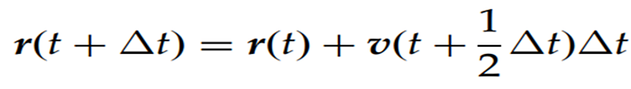
Velocity-Verlet Algorithm

A more advanced algorithm than the Leap-Frog method is called the Velocity-Verlet method. In this approach, the atomic positions and velocities at t + Δt/2 are obtained simultaneously from their values at time t and are calculated using the following equations:

Equation 8.

Equation 9.

Equation10.

The Velocity-Verlet algorithm addresses the main weakness of the Verlet and Leap-Frog algorithms, namely the definition of velocities (6).

Figure 4. Integration of the equations of motion using the Velocity-Verlet algorithm (6).

In conclusion, time integration algorithms are fundamental components that directly determine both the accuracy and computational efficiency of molecular dynamics simulations. Methods such as Verlet, Leap-Frog, and Velocity-Verlet offer different advantages in terms of numerical stability, energy conservation, and computational cost, and the choice of algorithm should be evaluated based on the simulation’s objective, system size, and thermodynamic conditions. While the classical Verlet method stands out for its simplicity and time reversibility, derivative algorithms that explicitly update velocities provide greater flexibility for temperature control and advanced sampling techniques. Therefore, there is no single “best” algorithm in molecular dynamics; the appropriate choice should be made by balancing speed and accuracy while considering the physical requirements of the simulation.

References

1. Cocklin, R., Heyen, J., Larry, T., Tyers, M., & Goebl, M. (2011). New insight into the role of the Cdc34 ubiquitin-conjugating enzyme in cell cycle regulation via Ace2 and Sic1. Genetics, 187(3), 701–715. https://doi.org/10.1534/genetics.110.125302

2. Papaleo, E., Casiraghi, N., Arrigoni, A. et al. (2012). Atomistic insights into the regulatory mechanisms mediated by post-translational modifications: molecular dynamics investigations. Curr. Phys. Chem. 2: 344–362.

3. Dror, R. O., Dirks, R. M., Grossman, J. P., Xu, H., & Shaw, D. E. (2012). Biomolecular simulation: a computational microscope for molecular biology. Annual review of biophysics, 41, 429–452. https://doi.org/10.1146/annurev-biophys-042910-155245

4. Verlet, L. (1967) Computer “Experiments” on Classical Fluids. I. Thermodynamical Properties of Lennard-Jones Molecules. Physical Review, 159, 98–103.https://doi.org/10.1103/PhysRev.159.98

5. Zhou K., Liu B. “Molecular Dynamic Simulation: Fundamentals and Applications” Elsevier 2022. https://doi.org/10.1016/C2017-0-04711-0

6. Boisseau P., Houdy P., Lahmani M. “Nanoscience Nanobiotechnology and Nanobiology” Springer-Verlag Berlin Heidelberg 2009. https://doi.org/10.1007/978-3-540-88633-4